QL-500A
FAQs & Troubleshooting |
When I use the Excel Add-In with my address data, the address is not displayed in the correct format. Each Excel column is printed on a separate line.
The Excel add-in is designed for simple printing of information without any complicated formatting. Therefore, if you need to place the data of two or more columns on the same line, another method needs to be used to achieve this.
There are two ways to print your addresses correctly from Excel:
- Use the "CONCATENATE" function in Excel to combine the information in the cells together.
- Load your Excel address data directly within P-touch Editor, join the required fields together, and print directly from P-touch Editor (do not use the Excel Add-In).
DETAIL OF PROBLEM
Each Excel column is printed as a separate line on your label. So if we take this example of an address stored in Excel:

When the text is highlighted (A2 to F2), the P-touch Add-In icon is clicked, the text on the label will be placed as follows:

You need to combine the text in the Excel columns into the correct order.
There are two ways to achieve this – by combining the text in Excel and using the Excel Add-In to print, or by combining the text in P-touch Editor before printing directly from the editor program.
METHOD #1 – USING EXCEL WITH THE EXCEL ADD-IN
To combine the text in Excel, we use the "CONCATENATE" function. Using our example Excel data again:

we need to combine the first three columns into one line. To do this, we would use the following Excel command in cell G2:
=CONCATENATE(A2," ",B2," ",C2)
Because cell A2 contains "Mr", cell B2 contains "John" and cell C2 contains "Smith", the concatenate command as shown above will produce:
Mr [SPACE] John [SPACE] Smith (the space is created by placing a space between two quotation marks - " ").
So, by moving our cursor to cell reference G2, and using this function we get:

Repeat this in the other columns (H2, I2, J2 etc), or if we do not need to join the columns together, simply use the command to copy what is in the other cell (for example, use the command "=D2").
Now that our data is in the correct order, we can are able to highlight these new cells, and then click on the P-touch Add-In icon to make the address label appear correctly:


To repeat the same procedure on all the other rows of data, simply highlight the new cells we have created (in this example, G2 to I2), and copy/paste them in the other rows:


Whenever using the P-touch Add-In for Excel, highlight the data in the new columns we have created (columns G, H and I), and the label will print correctly.
METHOD #2 – USING THE JOIN FIELDS OPTION IN P-TOUCH EDITOR
By loading your Excel sheet with your addresses, you can join the data in certain fields (columns) so they appear next to each other on your label.
This example shows how to join the multiple fields together and print your labels.
Of course, with this function you can join any fields (columns) together to make your data appear in the correct order.
-
Preparing the database.
In this example, we will create the same style labels as the above-described label using the following Excel data again.

-
Connecting the database
- Click [File] - [Database] - [Connect...]
-
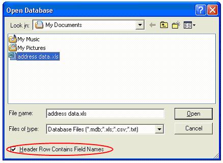
Find the directory and select the prepared Excel file.
Make sure that there is a check mark in the "Header Row Contains Field Names" check box in the Open Database dialog box.
If the file being used contains multiple sheets, the Select Table dialog box appears. Select the sheet that you wish to link to the layout.
-
Joining fields
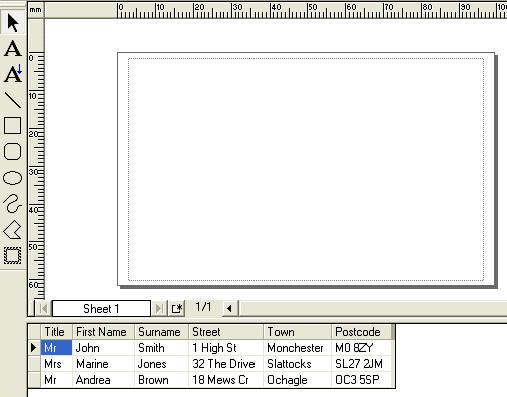
Joining the six fields together:- Click on the database window (the connected database) to display "Database" on the menu bar.
-
Click [Database] - [Connect Fields...]
The "Define Joined Fields" dialog box appears.

-
Click
 .
. -
The "Add a Joined Field" dialog box appears.

-
In the "Fields:" list box, select the "Title" field and then click
 .
.

-
In the same way, select the "First name" field and then click .
Repeat the same steps until all fields have been selected.
In edit box, insert a space after [Title], [First name] and [Town], and type "\n" before and after [Street] as follows:
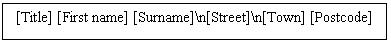
Entering "\n" enables you to create a new line.
-
Click
 .
.

-
The "Define Joined Fields" dialog box appears, showing the joined fields.
Click .
.
-
Merging text into a layout
- Click [Database] - [Merge into Layout...] or [Insert] - [Database field].
-
The "Merge fields" dialog box appears.
Select "Text" from the "Merge Type" pull-down menu and select "[Title] [First name] [Surname]\n[Street]\n[Town] [Postcode]" from the "Database Fields that Can Be Merged" list box.

-
Click
 .
. -
Now the six fields of [Title], [First name], [Surname], [Street], [Town] and [Postcode] joined together have been merged.

-
Adjusting the merged data.
Adjust the height, size and position of the merged object.


You can easily adjust the text size in the object by using the and
and  buttons.


Refer to the FAQ: "I want to create name badges by joining "First Name" and "Last Name" fields together." -
Printing
- Click [File] - [Print...].
- The Print dialog box appears.
-
Under "Print Range", select the desired print range.

-
Click
 .
.For details on selecting a record range, refer to the following table.
Printing Range Data of Printing Subject All Records Designates all records. Current Record Designate the currently displayed record. Selected Record(s) Designates the record currently selected in the database window. Record Range Designates the record range designated in "From" and "To".